Momentum, Curveball, and Nesterov Acceleration

This post explores some relationships between the recent Curveball optimization method (https://arxiv.org/abs/1805.08095, more recent version at https://openreview.net/forum?id=Sygx4305KQ) and Nesterov momentum (as popularized by http://proceedings.mlr.press/v28/sutskever13.html).

Suppose we are iteratively optimizing a scalar-valued function $f(x)$ wrt $x$ by gradient descent. We wish to take a step $z$ that minimizes $f(x + z)$, whose Taylor series is given by

$$f(x + z) = f(x) + z^\top f'(x) + \frac{1}{2} z^\top f''(x) z + \ldots$$

where $f'(x)$ denotes the gradient of $f$ evaluated at $x$, and similarly $f''(x)$ is the Hessian. Second-order methods locally model $f(x)$ by a second-order approximation $\hat{f}$:

$$\hat{f}(x + z) = f(x) + z^\top f'(x) + \frac{1}{2} z^\top f''(x) z,$$

according to which the optimal step is

$$z^\star = \operatorname{argmin}_z f(x) + z^\top f'(x) + \frac{1}{2} z^\top f''(x) z = (f''(x))^{-1} f'(x).$$

However, multiplying by the inverse Hessian is expensive.

The authors of Curveball propose instead to solve for $z^\star$ by gradient descent, and to interleave this inner optimization with the outer optimization over $x$:

\begin{align}
z &\leftarrow \rho z - \beta \frac{\partial \hat{f}(x + z)}{\partial z} \\
x &\leftarrow x + z
\end{align}

where $\rho, \beta$ are hyperparameters.

Now $\frac{\partial \hat{f}(x + z)}{\partial z} = f'(x) + f''(x) z$; if the approximation $\hat{f}$ were first-order instead, the $f''(x) z$ term would disappear and this would be equivalent to classical momentum.

But if we're going to use gradients to optimize $z$, then why make the second-order approximation at all? Why not let $\hat{f} = f$ and optimize the step $z$ to minimize $f(x + z)$:

\begin{align}
z &\leftarrow \rho z - \beta \frac{\partial f(x + z)}{\partial z} \\
x &\leftarrow x + z
\end{align}

By a change of variables $y = x + z$, the derivative $\frac{\partial f(x + z)}{\partial z} = \frac{\partial f(y)}{\partial y} \frac{\partial y}{\partial z}$ is simply $f'(x + z)$. From this it is easy to see that this update rule is practically equivalent to that for Nesterov momentum given in Sutskever et al 2013:

\begin{align}
z &\leftarrow \rho z - \beta f'(x + \rho z) \\ x &\leftarrow x + z.
\end{align}

The only difference is the weighting by $\rho$ of the tentative step in the evaluation point $x + \rho z$ of $f'$.

What does that mean? It means that if classical momentum is first-order and Curveball is second-order, well then Nesterov momentum is the infinite-order version of momentum. It's tempting to conclude that Curveball is a worse version of Nesterov momentum, as it makes an unnecessary second-order approximation. However, the Curveball paper goes on to adopt all the usual second-order tricks (GGN, trust region, etc.). It's unclear how the final algorithm performs relative to Nesterov momentum.

On the Variance of Unbiased Online Recurrent Optimization

This blog post summarizes the brand new paper On the Variance of Unbiased Online Recurrent Optimization (Cooijmans & Martens, 2019), an extensive investigation into the UORO (Tallec & Ollivier, 2017) algorithm for online training of recurrent neural networks. The work was done in close collaboration with James Martens, who supervised me during my internship at DeepMind where the work started.

I'm excited about this work; what seemed like a simple problem -- effective forward-mode differentiation -- turned out to be a rich source of deeply interesting connections and possibilities.

Differentiation through time

We'll consider a general class of differentiable recurrent models with state $h_t$ governed by:
$$
h_t = F (h_{t - 1}, x_t ; \theta_t) .
$$
Here $x_t$ is an observation made at time $t$, and $\theta_t$ are the RNN's parameters (e.g. weight matrix). As usual, the parameters are shared over time, i.e. $\theta_t = \theta$; having the subscript $t$ on the parameters $\theta$ conveniently lets us refer to the partial derivatives $\frac{\partial h_t}{\partial \theta}$ by the total derivative $\frac{\mathrm{d} h_t}{\mathrm{d} \theta_t}$. We will generally use the notation $\mathcal{J}^{y}_{x}$ for the (total) Jacobian matrix of $y$ with respect to $x$.

State propagation through an RNN

At each step, the RNN incurs a loss $L_t$ which is a differentiable function of the hidden state $h_t$. In order to optimize $\theta$ to minimize the total loss $L = \sum_{t = 1}^T L_t$ over a sequence of length $T$, we require an estimate of the gradient $\mathcal{J}^L_{\theta}$.
$$
\mathcal{J}^L_{\theta} = \sum_{t = 1}^T \sum_{s = 1}^T
   \mathcal{J}^{L_t}_{\theta_s} = \underbrace{\sum_{s = 1}^T \left( \sum_{t =
   s}^T \mathcal{J}^{L_t}_{h_s} \right)
   \mathcal{J}^{h_s}_{\theta_s}}_{\text{reverse accumulation}} =
   \underbrace{\sum_{t = 1}^T \mathcal{J}^{L_t}_{h_t} \left( \sum_{s = 1}^t
   \mathcal{J}^{h_t}_{\theta_s} \right)}_{\text{forward accumulation}}
$$
Each of the terms $\mathcal{J}^{L_t}_{\theta_s}$ indicates how the use of the parameter $\theta$ at time $s$ contributed to the loss at time $t$. The triangular/causal structure $\mathcal{J}^{L_t}_{\theta_s} =\mathbb{1}_{s \leqslant t} \mathcal{J}^{L_t}_{\theta_s}$ allows two useful factorizations of the double sum.

The first, labeled reverse accumulation, is used by the popular Backpropagation Through Time algorithm (BPTT). In BPTT we run the model forward to compute the activations and losses, and subsequently run backward to propagate gradient $\mathcal{J}^L_{h_t}$ back through time:
$$
\mathcal{J}^L_{h_t} =\mathcal{J}^L_{h_{t + 1}} \mathcal{J}^{h_{t +
   1}}_{h_t} +\mathcal{J}^{L_t}_{h_t} .
$$
By following this recursion, we can aggregate the terms $\mathcal{J}^L_{\theta_t} =\mathcal{J}^L_{h_t} \mathcal{J}^{h_t}_{\theta_t}$ to compute the gradient. The backpropagation $\mathcal{J}^L_{h_{t + 1}} \mathcal{J}^{h_{t + 1}}_{h_t}$ is a vector-matrix product, which has the same cost as the forward propagation of state $h_t$ in a typical RNN.

Back-propagation of $\mathcal{J}^L_{h_t}$ by BPTT

The second factorization (forward accumulation) is used by the Real-Time Recurrent Learning algorithm (RTRL). The recursion
$$
\mathcal{J}^{h_t}_{\theta} =\mathcal{J}^{h_t}_{h_{t - 1}} \mathcal{J}^{h_{t
   - 1}}_{\theta} +\mathcal{J}^{h_t}_{\theta_t}
$$
is chronological and can be computed alongside the RNN state. Given $\mathcal{J}^{h_t}_{\theta}$, we can compute the term $\mathcal{J}^{L_t}_{\theta} =\mathcal{J}^{L_t}_{h_t} \mathcal{J}^{h_t}_{\theta}$ and immediately update the parameter $\theta$ (with some technical caveats). The drawback is that the forward propagation $\mathcal{J}^{h_t}_{h_{t - 1}} \mathcal{J}^{h_{t - 1}}_{\theta}$ is an expensive matrix-matrix product. Whereas BPTT cheaply propagated a vector $\mathcal{J}^L_{h_t}$ of the same size as the RNN state, RTRL propagates a matrix $\mathcal{J}^{h_t}_{\theta}$ that consists of one parameter-sized vector for each hidden state. Since typically the parameter is quadratic in the size of the hidden state, this is cubic, and the forward-propagation is quartic (i.e. for a meager 100 hidden units, RTRL is 10,000 times more expensive than BPTT!).

Forward-propagation of $\mathcal{J}^{h_t}_{\theta}$ by RTRL

It is important to note that the jacobians involved in these recursions depend on the activations $h_t$ and other intermediate quantities. In RTRL, these quantities naturally become available in the order in which they are needed, after which they may be forgotten. BPTT revisits these quantities in reverse order, which requires storing them in a stack.

This is the main drawback of BPTT: its storage grows with the sequence length $T$, which limits the temporal span of dependencies it can capture (as in truncated BPTT) and the rate at which parameter updates can occur.

RTRL has some things to recommend it, if only we had a way of dealing with that giant matrix $\mathcal{J}^{h_t}_{\theta}$.

Unbiased Online Recurrent Optimization

UORO (Tallec & Ollivier, 2017) approximates RTRL by maintaining a rank-one estimate of $\mathcal{J}^{h_t}_{\theta}$ using random projections. A straightforward derivation starts from the expression
$$
\mathcal{J}^{h_t}_{\theta} = \sum_{s \leqslant t} \mathcal{J}^{h_t}_{h_s}
   \mathcal{J}^{h_s}_{\theta_s} .
$$
Into each term, we insert a random rank-one matrix $\nu_s \nu_s^{\top}$ with expectation $\mathbb{E} [\nu_s \nu_s^{\top}] = I$ (e.g. random signs):
$$
\mathcal{J}^{h_t}_{\theta} \approx \sum_{s \leqslant t}
   \mathcal{J}^{h_t}_{h_s} \nu_s \nu_s^{\top} \mathcal{J}^{h_s}_{\theta_s} .
$$
The random projections onto $\nu_s$ serve the compress the matrices $\mathcal{J}^{h_t}_{h_s}$ and $\mathcal{J}^{h_s}_{\theta_s}$ into vector-sized quantities. But accumulating this sum online is still expensive: we must either accumulate the matrix-sized quantities $\mathcal{J}^{h_t}_{h_s} \nu_s \nu_s^{\top} \mathcal{J}^{h_s}_{\theta_s}$ or the sequence of pairs of vectors $\mathcal{J}^{h_t}_{h_s} \nu_s$, $\nu_s^{\top} \mathcal{J}^{h_s}_{\theta_s}$.

We can pull the same trick again and rely on noise to entangle corresponding pairs. Let $\tau$ be a random vector with expectation $\mathbb{E} [\tau \tau^{\top}] = I$. Then
$$
\mathcal{J}^{h_t}_{\theta} \approx \sum_{s \leqslant t}
   \mathcal{J}^{h_t}_{h_s} \nu_s \nu_s^{\top} \mathcal{J}^{h_s}_{\theta_s} =
   \sum_{s \leqslant t} \mathcal{J}^{h_t}_{h_s} \nu_s \tau_s \tau_s
   \nu_s^{\top} \mathcal{J}^{h_s}_{\theta_s} \approx \left( \sum_{s \leqslant
   t} \mathcal{J}^{h_t}_{h_s} \nu_s \tau_s \right) \left( \sum_{s \leqslant t}
   \tau_s \nu_s^{\top} \mathcal{J}^{h_s}_{\theta_s} \right) .
$$
For simplicity, we will replace the independent noise variables $\tau_t,\nu_t$ by a single random vector $u_t = \tau_t \nu_t$.

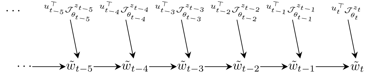
Now we have two vector-valued sums, which we can efficiently maintain online:
\begin{align}
  \tilde{h}_t & = \mathcal{J}^{h_t}_{h_{t - 1}} \tilde{h}_{t - 1} + u_t \\
  \tilde{w}_t^{\top} & = \tilde{w}_{t - 1}^{\top} + u_t^{\top}
  \mathcal{J}^{h_t}_{\theta_t} .
\end{align}
This joint recursion is similar to that for $\mathcal{J}^{h_t}_{\theta}$ in RTRL; the approximation $\tilde{h}_t \tilde{w}_t^{\top}$ is used as a rank-one stand-in for $\mathcal{J}^{h_t}_{\theta}$. Notice how the unwieldy matrix-matrix product in RTRL has been replaced by a cheap matrix-vector product $\mathcal{J}^{h_t}_{h_{t - 1}} \tilde{h}_{t - 1}$: UORO is as cheap as BPTT.

Forward-propagation of noise in UORO

Accumulation of back-propagated noise in UORO

So that's the basic workings of UORO: randomly project in state space and then randomly project once again in time. Both of these projections introduce errors in the approximation $\mathcal{J}^{h_t}_{\theta} \approx \tilde{h}_t \tilde{w}_t^{\top}$, due to connecting the wrong elements together in the matrix-matrix product $\mathcal{J}^{h_t}_{h_s} \mathcal{J}^{h_s}_{\theta_s}$ (*spatial* cross-terms) and due to connecting the wrong time steps $q \neq r$ together in $\mathcal{J}^{h_t}_{h_r} \nu_r \nu_q^{\top} \mathcal{J}^{h_q}_{\theta_q}$ (*temporal* cross-terms). In expectation, these errors cancel out and the approximation is unbiased.

Variance reduction through iterative rescaling

UORO came with a variance reduction technique that iteratively rescales all quantities involved:
\begin{align}
  \tilde{h}_t & = \gamma_t \mathcal{J}^{h_t}_{h_{t - 1}} \tilde{h}_{t - 1} +
  \beta_t u_t\\
  \tilde{w}_t^{\top} & = \gamma_t^{- 1} \tilde{w}_{t - 1}^{\top} +
  \beta_t^{- 1} u_t^{\top} \mathcal{J}^{h_t}_{\theta_t} .
\end{align}
The coefficients $\gamma_t, \beta_t$ serve to reduce the norms of undesired temporal cross-terms (e.g. $\gamma_t \beta_t^{- 1} \mathcal{J}^{h_t}_{h_{t - 1}} \tilde{h}_{t - 1} u_t^{\top} \mathcal{J}^{h_t}_{\theta_t}$) while keeping corresponding terms (e.g. $\gamma_t \gamma_t^{- 1} \mathcal{J}^{h_t}_{h_{t - 1}} \tilde{h}_{t - 1} \tilde{w}_{t - 1}^{\top}$) unaffected. In practice it seems like the brunt of the work is done by $\gamma_t$, which distributes, across $\tilde{h}_t$ and $\tilde{w}_t$, the contraction of $\tilde{h}_{t - 1}$ due to forward propagation through $\mathcal{J}^{h_t}_{h_{t - 1}}$ (aka gradient vanishing).

In our paper we argue that this variance reduction scheme, although cheap and very effective, has some room for improvement. UORO's coefficients are chosen to minimize
$$
\mathbb{E}_{\tau_t} [\| \tilde{h}_t \tilde{w}_t^{\top} -
   (\mathcal{J}^{h_t}_{h_{t - 1}} \tilde{h}_{t - 1} \tilde{w}_{t - 1}^{\top} +
   u_t u_t^{\top} \mathcal{J}^{h_t}_{\theta_t}) \|^2_F],
$$
i.e. the expected norm of the error in $\tilde{h}_t \tilde{w}_t^{\top}$ as a rank-one approximation of the rank-two matrix $\mathcal{J}^{h_t}_{h_{t - 1}} \tilde{h}_{t - 1} \tilde{w}_{t - 1}^{\top} + u_t u_t^{\top} \mathcal{J}^{h_t}_{\theta_t}$. This is a natural quantity to target, but it ignores the bigger picture: downstream, the approximate Jacobians $\tilde{h}_t \tilde{w}_t^{\top} \approx \mathcal{J}^{h_t}_{\theta}$ are used to produce a sequence of gradient estimates $\mathcal{J}^{L_t}_{h_t} \tilde{h}_t \tilde{w}_t^{\top} \approx \mathcal{J}^{L_t}_{\theta}$, which are aggregated by some optimization process into a *total gradient estimate*
$$
\sum_{t \leqslant T} \mathcal{J}^{L_t}_{h_t} \tilde{h}_t \tilde{w}_t^{\top}
   \approx \sum_{t \leqslant T} \mathcal{J}^{L_t}_{\theta}
   =\mathcal{J}^L_{\theta} .
$$
Notice in particular that each of the terms $\mathcal{J}^{L_t}_{h_t} \tilde{h}_t \tilde{w}_t^{\top}$ is based largely on the same random quantities, which produces interactions between consecutive gradient estimates. In our paper we instead seek to minimize the *total variance*
$$
\mathbb{E}_u \left[ \| \sum_{t \leqslant T} \mathcal{J}^{L_t}_{h_t}
   \tilde{h}_t \tilde{w}_t^{\top} -\mathcal{J}^L_{\theta} \|^2 \right] .
$$
Since consecutive gradient estimates are not independent, the variance of the sum is not simply the sum of the variances.

Theoretical framework

We analyze a generalization of UORO's recursions:
\begin{align}
  \tilde{h}_t & = \mathcal{J}^{h_t}_{h_{t - 1}} \tilde{h}_{t - 1}
  +\mathcal{J}^{h_t}_{z_t} Q_t u_t\\
  \tilde{w}_t^{\top} & = \tilde{w}_{t - 1}^{\top} + u_t^{\top} Q_t^{- 1}
  \mathcal{J}^{z_t}_{\theta_t} .
\end{align}
The symbolic variable $z_t$ may refer to any cut vertex along the path from $\theta_t$ to $h_t$. In vanilla UORO, $z_t \equiv h_t$, so projection occurs in state space. Other choices include projection in parameter space ($z_t \equiv \theta_t$) and projection in preactivation space (which has convenient structure).

We also replaced the scalar coefficients $\gamma_t, \beta_t$ by matrices $Q_t$ (see the paper for the details). These matrices transform the noise vectors $u_t$; the section on REINFORCE below reveals an interpretation of these matrices as modifying the covariance of exploration noise.

We define the following shorthands:
\begin{align}
& b^{(t) \top}_s =\mathcal{J}^{L_t}_{z_s} & \text{and} & & J_s  = \mathcal{J}^{z_s}_{\theta_s}.
\end{align}
Now the total gradient estimate,
\begin{align}
\sum_{t \leqslant T} \mathcal{J}^{L_t}_{h_t} \tilde{h}_t \tilde{w}_t^{\top}
&= \sum_{t \leqslant T} \mathcal{J}^{L_t}_{h_t}
\left( \sum_{s \leqslant t} \mathcal{J}^{h_t}_{z_s} Q_s u_s \right)
\left( \sum_{s \leqslant t} u_s^{\top} Q_s^{-1} \mathcal{J}^{z_s}_{\theta_s} \right)
\\&= \left( \sum_{s \leqslant t} b^{(t)}_s Q_s u_s \right)
   \left( \sum_{s \leqslant t} u_s^{\top} Q_s^{-1} J_s \right)
,
\end{align}
can be expressed as
$$
\sum_{t \leqslant T} \left(\begin{array}{c}
     b^{(t)}_1\\
     \vdots\\
     b^{(t)}_T
   \end{array}\right)^{\top} \left(\begin{array}{ccc}
     Q_1 &  & \\
     & \ddots & \\
     &  & Q_T
   \end{array}\right) \left(\begin{array}{c}
     u_1\\
     \vdots\\
     u_T
   \end{array}\right) \left(\begin{array}{c}
     u_1\\
     \vdots\\
     u_T
   \end{array}\right)^{\top} \left(\begin{array}{ccc}
     Q_1 &  & \\
     & \ddots & \\
     &  & Q_T
   \end{array}\right)^{- 1} \left(\begin{array}{ccc}
     S^{(t)}_1 &  & \\
     & \ddots & \\
     &  & S^{(t)}_T
   \end{array}\right) \left(\begin{array}{c}
     J_1\\
     \vdots\\
     J_T
   \end{array}\right),
$$
where $S^{(t)}_s =\mathbb{1}_{s \leqslant t} I$ enforces causality: the estimate $\mathcal{J}^{L_t}_{h_t} \tilde{h}_t \tilde{w}_t^{\top}$ at time $t$ does not involve contributions $\mathcal{J}^{z_s}_{\theta_s}$ from future ($s > t$) parameter applications. This property already holds on the $b$ side, as $b^{(t)}_s =\mathbb{1}_{s \leqslant t} b^{(t)}_s$.

Giving names to these concatenated quantities, we may write
$$
  \sum_{t \leqslant T} \mathcal{J}^{L_t}_{h_t} \tilde{h}_t \tilde{w}_t^{\top}
 = \sum_{t \leqslant T} b^{(t) \top} Q u u^{\top} Q^{- 1} S^{(t)} J.
$$
This is a fairly simple expression, which makes it easy to analyze the behavior of the estimator. We see immediately that the estimator is unbiased, as $\mathbb{E}_u [Q u u^{\top} Q^{- 1}] = Q\mathbb{E}_u [u u^{\top}] Q^{- 1} = Q Q^{- 1} = I$ ($Q$ is assumed to be independent of the noise $u$). In the paper we also derive the variance; for this blog post it will be enough to note that it is dominated by a product of traces,
$$
V (Q) = \sum_{s \leqslant T} \sum_{t \leqslant T} \operatorname{tr} \left( \sum_{r
   \leqslant T} b^{(s)}_r b_r^{(t) \top} Q_r Q_r^{\top} \right) \operatorname{tr}
   \left( \sum_{q \leqslant T} S^{(t)}_q J_q J_q^{\top} S^{(s)}_q (Q_q
   Q_q^{\top})^{- 1} \right) .
$$

Toward improved variance reduction

We wish to minimize this wrt $Q$, but in a way that corresponds to a practical algorithm. We investigate the case where $Q$ has the form $Q_t = \alpha_t Q_0$ for scalar coefficients $\alpha_t$ and a constant $Q_0$ matrix. Intuitively, the $\alpha_t$ could be chosen by an iterative rescaling rule similar to the $\gamma_t, \beta_t$ scheme from UORO, while $Q_0$ would be based on supposedly slow-moving second-order information.

Joint optimization of these quantities turned out to be analytically intractable, and even alternately optimizing the $\alpha_t$ and $Q_0$ is difficult. Still, we made some headway on these problems; of particular interest is the quantity
$$
B = \sum_{s \leqslant T} \sum_{t \leqslant T} \left( \sum_{q = 1}^{\min (s,
   t)} \alpha_q^{- 2} \| a_q \|^2 \right) \left( \sum_{r \leqslant T}
   \alpha_r^2 b^{(s)}_r b^{(t) \top}_r \right) = \sum_{q \leqslant T} \sum_{r
   \leqslant T} \frac{\alpha_r^2}{\alpha_q^2} \| a_q \|^2 \left( \sum_{s =
   q}^T b^{(s)}_r \right) \left( \sum_{t = q}^T b^{(t)}_r \right)^{\top},
$$
which gives the optimal $Q_0$ as $Q_0 = B^{- 1 / 4}$ when projection occurs in preactivation space (see the paper). The vector $a_t$ is the input to the RNN (i.e. the previous state, the current observation and a bias), which shows up here due to the convenient structure of the backward Jacobian $J_t = \mathcal{J}^{z_t}_{\theta_t} = I \otimes a_t^{\top}$ in the case of
preactivation-space projection.

In the optimal case $Q_0 = B^{- 1 / 4}$, the variance contribution $V (Q)$ above reduces from $\operatorname{tr} (B) \operatorname{tr} (I)$ to $\operatorname{tr} (B^{1 / 2})^2$, which by Cauchy-Schwarz is an improvement to the extent that the eigenspectrum of $B$ is lopsided rather than flat. We show empirically, in a small-scale controlled setting in which $B$ is known (by backprop), that the optimal (in our framework) $\alpha_t$ and $Q_0$ result in significant variance reduction.

Of course, it is not obvious how to implement these ideas effectively. The theoretically optimal choices for these quantities depend on information that is unknown. For instance, the matrix $B$ is sort of a weighted covariance of sums of future gradients $\sum_{s = q}^T b^{(s)}_r$; if we knew these gradients we wouldn't need to maintain the RTRL Jacobian $\mathcal{J}^{h_t}_{\theta}$ in the first place! One cool idea is to estimate it online using the same rank-one tricks we use to estimate the gradient, which results in a self-improving algorithm. We show one such estimator, but it (and others like it) fared poorly in practice, as one might have guessed.

However, the theory is meant to guide practice, not to dictate it. Unbiased estimation of $B$ is not necessary (as the overall algorithm is unbiased for any $Q_0$), and nor is it particularly desirable if it comes at the cost of injecting more noise into the system. It is well-known from optimization that second-order information is hard to estimate reliably in the stochastic setting. Most likely there exist heuristic choices of $Q_0$ (guided by the theory) that enable variance reduction without introducing additional noise variables and which may be more amenable to noisy estimation in the first place.

Projecting in preactivation space

As also discovered by Mujika et al. (2018), it is usually possible to do away with random projection onto spatial noise vectors $\nu_t$ altogether. The trick is that the gradient contribution $\mathcal{J}^L_{\theta_t}$ due to application of the parameter $\theta$ at time $t$ is already rank-one if the parameter plays the role of a weight matrix (as it almost always does). E.g. if the recurrent neural network takes the form
$$
p_t = W_t a_t \\
h_t = f (p_t)
$$
such that $\theta_t = \operatorname{vec} (W_t)$ and with $a_t = \left(\begin{array}{ccc}
  h_{t - 1}^{\top} & x_t^{\top} & 1 \end{array}\right)^{\top}$ being the concatenated input to the RNN at time $t$, then the gradient with respect to $W_t$ is just the outer product of
the gradient with respect to the preactivations $p_t$ and the inputs $a_t$:
$$
\nabla_{W_t} L = (\mathcal{J}^L_{p_t})^\top a_t^\top
$$
The notation becomes a bit of a trainwreck when we switch to working with the vectorization $\theta_t = \operatorname{vec}(W_t)$ in order to speak of the Jacobians $\mathcal{J}^{h_t}_{\theta_t}$. Let's switch to Kronecker products for \otimes' sake:
$$
\mathcal{J}^{h_t}_{\theta_t} = \mathcal{J}^{h_t}_{p_t} (I \otimes a^{\top})
$$
This is formally a matrix, but it's more naturally thought of as a third-order $H \times P \times A$ tensor with elements $\frac{\partial h_{t i}}{\partial p_{t j}} a_{t k}$. ($H$, $P$, $A$ are the dimensions of $h_t$, $p_t$ and $a_t$ respectively.)

The key observation is that this third-order tensor can be broken up into an outer product of an $H \times P$ matrix $\mathcal{J}^L_{p_t}$ and an $A$-dimensional vector $a_t$ without any random projection. Plain UORO on the other hand would stochastically break it up into an outer product of an $H$-dimensional vector $\mathcal{J}^{h_t}_{p_t} u_t$ and a vectorized $P \times A$ matrix $u_t^\top \mathcal{J}^{p_t}_{\theta_t} = u_t^\top (I \otimes a_t^\top) = \operatorname{vec}(u_t a_t^\top)$. Although the factorization without projection does not introduce extra variance, it does introduce extra computation, as we are now propagating a matrix again as in RTRL (albeit a smaller one).

Now the approximate Jacobian takes the form $\tilde{H}_t (I \otimes \tilde{a}_t) \approx \mathcal{J}^{h_t}_{\theta}$, with $\tilde{H}_t$ and $\tilde{a}_t$ maintained according to
\begin{align}
  \tilde{H}_t & = \gamma_t \mathcal{J}^{h_t}_{h_{t - 1}} \tilde{H}_{t - 1} +
  \beta_t \tau_t \mathcal{J}^{h_t}_{p_t} \\
  \tilde{a}_t & = \gamma_t^{- 1} \tilde{a}_{t - 1} +
  \beta_t^{- 1} \tau_t a_t .
\end{align}
These are similar to UORO's recursions, except that the Jacobian factors $\mathcal{J}^{h_t}_{p_t}$ and $I \otimes a_t^\top$ are not projected onto noise vectors $u_t$ but rather multiplied by random signs $\tau_t$ before being accumulated into their respective sums.

Each gradient $\mathcal{J}^{L_t}_{\theta}$ is estimated by $\mathcal{J}^{L_t}_{h_t} \tilde{H}_t (I \otimes \tilde{a}_t) = \operatorname{vec} ( (\mathcal{J}^{L_t}_{h_t} \tilde{H}_t)^\top \tilde{a}_t^\top)$, which can still be computed without explicitly forming $\tilde{H}_t (I \otimes \tilde{a}_t^\top)$.

Forward-propagation of noise in preactivation space

Accumulation of activations

We show in the paper that this property can be exploited to reduce the variance contribution $V (Q)$ by a factor equal to the dimension of the preactivations, at the cost of increasing the computational complexity by the same factor. Typically, this means going from $\mathcal{O} (H^2)$ time (vanilla UORO) to $\mathcal{O} (H^3)$ time (preactivation-space UORO); a serious increase but still better than RTRL's $\mathcal{O} (H^4)$ time ($H$ is the size of the hidden state $h_t$).

The group that discovered this algorithm around the same time (the aforementioned Approximating Real-Time Recurrent Learning with Random Kronecker Factors (Mujika et al 2018)) released a new paper a few days ago, Optimal Kronecker-Sum Approximation of Real Time Recurrent Learning (Benzing et al 2019). I haven't had time to read it in full, but it looks like they found a way to optimize the low-rank approximation without biasing the approximation.

A link to REINFORCE

Finally, we show a near-equivalence between REINFORCE and UORO when the former is used to train a stochastic RNN with the following recurrent structure:
$$
h_t = F (\bar{h}_{t - 1}, x_t ; \theta_t) \\
\bar{h}_t = h_t + \sigma Q_t u_t
$$
Here $u_t \sim \mathcal{N} (0, I)$ is additive Gaussian noise, and $\sigma$ determines the level of noise. The invertible matrix $Q_t$ transforms the standard normal noise $u_t$ and corresponds to a covariance matrix, but the reason it is included here is because it will end up playing the same role as the $Q_t$ matrix discussed in the variance reduction section above. Effectively, the stochastic hidden state $\bar{h}_t \sim \mathcal{N} (h_t, \sigma^2 Q_t Q_t^{\top})$ is sampled from a Gaussian distribution centered on the deterministic hidden state $h_t$. We assume the loss $L_t$ to be a differentiable function of $\bar{h}_t$.

RNN with state perturbation

To be clear, the sole purpose of injecting this noise is so that we may apply REINFORCE to estimate gradients through the system and compare these estimates to those of UORO. The stochastic transition distribution will be our policy from the REINFORCE perspective, which suggests actions $\bar{h}_t$ given states $h_t$. We compute the REINFORCE estimator by running the stochastic RNN forward, thus sampling a trajectory of states $\bar{h}_t$, and at each step computing
$$
L_t \nabla_{\theta} \log p (\bar{h}_t | \bar{h}_0, \bar{h}_1 \ldots
   \bar{h}_{t - 1} ; \theta) \approx \mathcal{J}^{L_t}_{\theta} .
$$
The estimate consists of the loss $L_t$ times the score function of the trajectory. Intuitively, higher rewards (equivalently, lower losses) "reinforce" directions in parameter space that bring them about.

The score function $\bar{w}_t^{\top} = \nabla_{\theta} \log p (\bar{h}_t | \bar{h}_0, \bar{h}_1 \ldots \bar{h}_{t - 1} ; \theta)$ is maintained online according to
$$
\bar{w}_t^{\top} = \bar{w}_{t - 1}^{\top} + \nabla_{\theta} \log p
   (\bar{h}_t | \bar{h}_{t - 1} ; \theta_t) = \bar{w}_{t - 1} +
   \frac{1}{\sigma} u_t^{\top} Q_t^{- 1} \mathcal{J}^{h_t}_{\theta_t},
$$
which is analogous to $\tilde{w}$ in UORO. An important difference is that the backward Jacobians $\mathcal{J}^{h_t}_{\theta_t}$ are evaluated in the noisy system. In the paper we eliminate this difference by passing to the limit $\sigma \rightarrow 0$, which simulates the common practice of annealing the noise.

Besides $\tilde{w}_t$, UORO's estimate of $\mathcal{J}^{L_t}_{h_t} \tilde{h}_t \tilde{w}_t^{\top} \approx \mathcal{J}^{L_t}_{\theta}$ involves $\mathcal{J}^{L_t}_{h_t} \tilde{h}_t$. In REINFORCE, the inner product of $\bar{w}_t$ with this quantity is implicit in the multiplication by the loss. We can reveal it by taking the Taylor series of the loss around the point $u = 0$ where the noise is zero:
$$
L_t = L_t |_{u = 0} + \left( \sum_{s \leqslant t} \mathcal{J}^{L_t}_{u_s}
   |_{u = 0} u_s \right) + \frac{1}{2} \left( \sum_{r \leqslant t} \sum_{s
   \leqslant t} u_r^{\top} \mathcal{H}^{L_t}_{u_r, u_s} |_{u = 0} u_s \right)
   + \cdots
$$
Using the fact that derivatives with respect to $u_s$ are directly related to derivatives with respect to $h_s$, namely
$$
\mathcal{J}^{L_t}_{u_s} |_{u = 0} = \sigma \sum_{s \leqslant t}
   \mathcal{J}^{L_t}_{h_s} |_{u = 0} Q_s,
$$
we may write
$$
L_t = L_t |_{u = 0} + \sigma \mathcal{J}^{L_t}_{h_t} \left( \sum_{s
   \leqslant t} \mathcal{J}^{h_t}_{h_s} |_{u = 0} Q_s u_s \right) +\mathcal{O}
   (\sigma^2) .
$$
Plugging these into the REINFORCE estimate $L_t \nabla_{\theta} \log p (\bar{h}_t | \bar{h}_0, \bar{h}_1 \ldots \bar{h}_{t - 1} ; \theta)$, we get
$$
L_t \bar{w}_t^{\top} = \frac{1}{\sigma} L_t |_{u = 0} \left( \sum_{s
   \leqslant t} u_s^{\top} Q_s^{- 1} \mathcal{J}^{h_s}_{\theta_s} \right)
   +\mathcal{J}^{L_t}_{h_t} \left( \sum_{s \leqslant t}
   \mathcal{J}^{h_t}_{h_s} |_{u = 0} Q_s u_s \right) \left( \sum_{s \leqslant
   t} u_s^{\top} Q_s^{- 1} \mathcal{J}^{h_s}_{\theta_s} \right) +\mathcal{O}
   (\sigma^2) .
$$
When we pass to the limit $\sigma \rightarrow 0$, the second term becomes identical to the UORO estimate $\mathcal{J}^{L_t}_{h_t} \tilde{h}_t \tilde{w}_t^{\top}$. Note how the $Q_t$ matrices that determine the covariance of the exploration noise in REINFORCE play the exact same role as our variance reduction matrices in UORO.

The first term, which is zero in expectation, contributes infinite variance in the limit. In effect, annealing the noise deteriorates the quality of REINFORCE's estimates. This first term is usually addressed by subtracting a "baseline" -- an estimate of $L_t |_{u = 0}$ -- from the loss $L_t$ before multiplying with the score.

Conclusions

We've delved deeply into UORO, contributing a straightforward derivation, a general theoretical framework and a thorough analysis. Our proposed variance reduction using these $Q_t$ matrices is promising, although much work remains to be done. We've shown a variant of UORO that avoids the spatial level of stochastic approximation, thereby greatly reducing the variance at the cost of equally greatly increasing the time complexity. Finally, we have established a deep link between UORO and REINFORCE, which allows the interpretation of REINFORCE as an approximation to RTRL.